HCR – Less Than
Highlight Cell Rules - Less Than
With Excel’s preset conditional formatting tool, Highlight Cell Rules, you can alter a range of cells’ appearances according to your own criteria.
One of the choices for the condition is Less Than…
The Highlight Cell Rules section of the conditional formatting menu looks like this:
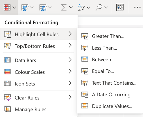
Highlight Cell Rule - Less Than Example
A cell with one of the appearance options will be highlighted by the “Less Than…” Highlight Cell Rule if the cell value is less than the value you have set.
It works with a text value as well as a number as the supplied value.
“55” will be the stated value in this case.

Any range can be selected as the one to which the Highlight Cell Rule should be applied. It could consist of a few cells, one row, one column, or a mix of several rows, columns, and cells.
Let’s use the Attack values to implement the rule.
“Less Than…” Emphasize Cell Rule, sequentially:
- Choose the D2:D8 range for Attack values.
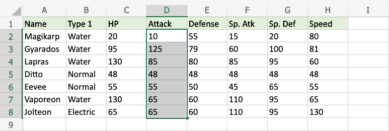
2. From the Home menu, select the Conditional Formatting icon in the ribbon.
3. Choose Highlight Cell Rules from the option that drops down.
4. Click on Less Than… in the menu.

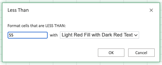
This will cause a dialog box to popup, allowing you to choose the appearance option and value.
5. In the input field, type 55.
6. From the dropdown menu, choose “Light Red Fill with Dark Red Text” as your appearance option.
Now, the cells with values less than “55” will be highlighted in red:
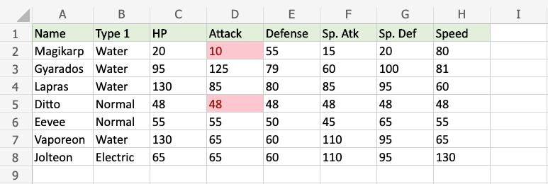
The only characters with Attack values less than 55 are Magikarp and Ditto; these values are indicated.
Note: Since the rule does not include the given number itself, Eevees’s Attack value of 55 is not noted.
Note: Manage Rules allows you to remove the Highlight Cell Rules.
Highlight Cell Rule - Less Than Example (with Text)
Text values can also be used with the “Less Than…” Highlight Cell Rule.
Excel will highlight text values beginning with a letter that appears earlier in the alphabet than the designated value using alphabetical order (A-Z).
“Electric” is the designated text value in this example.

Any range can be selected as the one to which the Highlight Cell Rule should be applied. It could consist of a few cells, one row, one column, or a mix of several rows, columns, and cells.
Now let’s use the Type 1 values to implement the rule.
“Less Than…” Emphasize Cell Rule, sequentially:
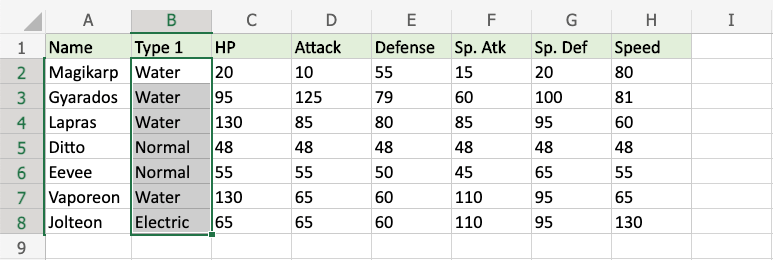
- To select Type 1 values, choose the range B2:B8.
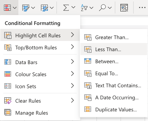
2. Click on the Conditional Formatting icon in the ribbon, from Home menu
3. Select Highlight Cell Rules from the drop-down menu
4. Select Less Than… from the menu
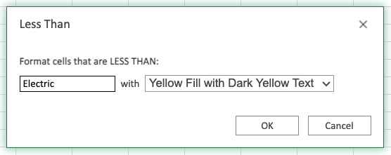
This will cause a dialog box to popup, allowing you to choose the appearance option and value.
5. In the input field, type Electric.
6. From the dropdown menu, choose “Yellow Fill with Dark Yellow Text” as the appearance choice.
Now, the cells with text values earlier in the alphabet than “Electric” will be highlighted in yellow:
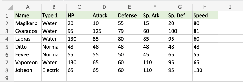
It appears like nothing has changed!
“W” stands for water, while “N” stands for normal.
Since Electric starts with “E” and “W” and “N” come later in the alphabet, none of them are highlighted.
Note: Because the rule only emphasizes text values that are higher in the alphabet, the supplied value “Electric” is likewise not highlighted.
What then becomes of the remaining letters in the text value?
What would happen if we added a made-up Pokemon with the following Name and Type?
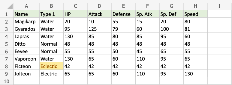
Observe that the highlighted type “Eclectic” belongs to the imaginary “Ficteon”.
From left to right, the Excel condition examines every letter in the given text value.
This is a Less Than and is emphasized because the “c” in “Eclectic” appears sooner in the alphabet than the “l” in “Electric”.
