Excel Conditional Format

Conditional Formatting

You can use conditional formatting to alter a range of cells’ appearances according to the circumstances you specify.

Rules based on predetermined numerical values or textual matching make up the conditions.

Cell appearance can be changed to visually draw attention to statistically significant data points.

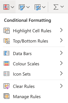
Excel’s browser version offers several pre-configured looks and conditions:

Note: Excel’s built-in conditional formatting options are limited in the online browser version.

You can create fully customized conditional formatting rules using the Excel application.

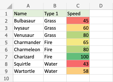
Here, the Speed values of each pokemon is formatted with a Color Scale:

Note: Excel offers a variety of color scale options.

Each Pokemon’s Speed statistics are highlighted using conditional formatting based on color scale.

Conditional formatting, step by step:

2. Click on the Conditional Formatting icon in the ribbon, from the Home menu
3. Select Color Scales from the drop-down menu

There are twelve Color Scale choices, each with a unique color variant.

The highest values will be represented by the color at the top of the icon .

4. Click on the “Green – Yellow – Red Colour Scale” icon

Now, the Speed value cells will have a colored background highlighting:

The highest values are represented by dark green, and the lowest by dark red.

Squirtle has the lowest speed value (43), whereas Charizard has the highest speed value (100).

Every cell in the range progressively turns from green to yellow to orange to red.