DSA Binary Trees
Binary Trees
A left child node and a right child node are the two maximum number of children that each node in a binary tree can have.
There are numerous advantages to this limitation, which states that a node may only have two child nodes:
- The comprehension, implementation, and execution speed of algorithms such as traversing, searching, insertion, and deletion improve.
- Searching is incredibly effective when the data is organized in a Binary Search Tree (BST).
- It is simpler to balance trees when there are fewer child nodes—an AVL Binary Tree, for instance—in the tree.
- Binary trees use less memory since they may be expressed as arrays.
See what a Binary Tree looks like and the terms we use to describe it by using the animation below.
=== example mukavu ===
In a Binary Tree, a node having one or two child nodes is called a parent node, or internal node.
The child node on the left is known as the left child node.
The child node on the right is the right child node.
The maximum number of edges that connect a root node to a leaf node is known as the tree height.
Binary Trees vs Arrays and Linked Lists
Advantages of Binary Trees over Linked Lists and Arrays
- Arrays are quick to access when an element, such as element 700 in an array of 1000 items, needs to be accessed directly. However, it takes time to insert and remove elements from memory because other elements must move to create room for the new element or to replace the deleted element.
- Linked Lists are quick to add or remove nodes; no memory shifting is required; nevertheless, accessing an element within the list requires traversing the list, which takes time.
- Binary Trees
When compared to arrays and linked lists, structures like binary search trees and AVL trees work well since they don’t require memory shifts and are quick when reading, removing, or inserting nodes.
On the following two pages, we will examine in more detail the operation of AVL Trees and Binary Search Trees (BSTs), but first, let’s examine how a Binary Tree can be implemented and navigated.
Types of Binary Trees
To better understand how Binary Trees might be organized, it is important to talk about the various variations, or types, of Binary Trees.
Since these terms and ideas will be utilized later in the lesson, it is also worthwhile to discuss the many types of Binary Trees at this time.
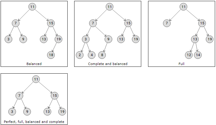
To make things as simple as possible, brief explanations of the many sorts of Binary Tree structures are provided below, along with illustrations of the structures.
For every node in the tree, a balanced binary tree has a maximum of one difference in height between its left and right subtrees.
Except for the final level, which can also be full or filled from left to right, every level in a complete binary tree is full with nodes. A complete binary tree’s features imply that it is balanced as well.
A complete binary tree is a tree type in which every node has two or zero offspring.
Every internal node in a perfect binary tree contains two child nodes, and every leaf node is on the same level, indicating that every level is full of nodes.A perfect binary tree has the qualities of being complete, balanced, and full.

Binary Tree Implementation
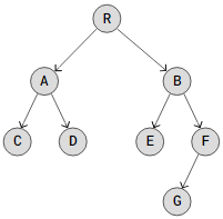
Let’s implement this Binary Tree:

The above Binary Tree can be constructed similarly to how we implemented a Singly Linked List, with the exception that we build a structure that allows each node to be linked to both its left and right offspring nodes, rather than just one next node.
One way to implement a Binary Tree is as follows:
Example
Python:
					class TreeNode:
    def __init__(self, data):
        self.data = data
        self.left = None
        self.right = None

root = TreeNode('R')
nodeA = TreeNode('A')
nodeB = TreeNode('B')
nodeC = TreeNode('C')
nodeD = TreeNode('D')
nodeE = TreeNode('E')
nodeF = TreeNode('F')
nodeG = TreeNode('G')

root.left = nodeA
root.right = nodeB

nodeA.left = nodeC
nodeA.right = nodeD

nodeB.left = nodeE
nodeB.right = nodeF

nodeF.left = nodeG

# Test
print("root.right.left.data:", root.right.left.data)
Binary Tree Traversal
Traversal is the process of going through a tree one node at a time, visiting each node.
There is only one clear way to traverse an array or linked list because they are linear data structures: begin at the first element, or node, and go through each one until you have seen them all.
However, there exist several methods for navigating through trees due to their non-linear branching.
Tree traversal techniques fall into two primary categories:
Breadth First Search (BFS) is the process of visiting nodes inside a level before moving on to the next level of the tree. This indicates a more lateral exploration of the tree.
Depth First Search (DFS) is a traversal technique that explores the tree branch by branch in a downward orientation, all the way down to the leaf nodes.
DFS traversals come in three different varieties:
- pre-order
- in-order
- post-order
The details of these three Depth First Search traversals are provided on the following pages.
