Quick Sort
For a general definition of time complexity, see this page.
Quicksort Time Complexity
The ‘pivot’ element is selected by the Quicksort algorithm, which then rearranges the other values to place the lower values on the left and the higher values on the right of the pivot element.
After that, the Quicksort algorithm keeps sorting the sub-arrays on both the left and right sides of the pivot element until the array is sorted recursively.
Worst Case
We can start by examining the worst case situation in order to get the time complexity for Quicksort.
If the array has already been sorted, that is the worst situation for Quicksort. In this case, each recursive call results in a single sub-array, and subsequent sub-arrays are always one element shorter than the preceding array.
Thus, Quicksort needs to make recursive calls to itself. n time, and it has to perform each time. n2. average comparisons.
The most difficult case time is:
===formula===
Average Case
Actually, Quicksort is substantially faster on average.
Because the array is divided roughly in half each time Quicksort executes recursively, the size of the sub-arrays decreases quickly, reducing the number of recursive calls required and allowing Quicksort to complete sooner than in the worst case scenario. This is why Quicksort is fast on average.
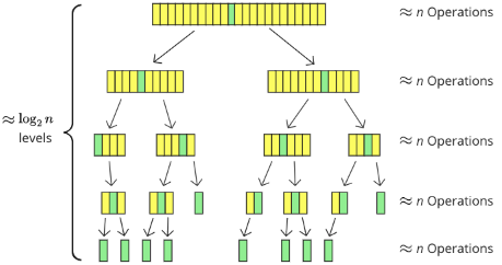
The Quicksort sorting process divides an array of 23 items into smaller arrays, as seen in the image below.

After moving the pivot element (green) to the center, the array is divided into sub-arrays (yellow). Each of the five recursion levels’ progressively smaller sub-arrays touches around n values in some way, either by comparison, movement, or both.
log2 tells us how many times a number can be split in 2, so log2 is a good estimate for how many levels of recursions there are. log2(23)≈4.5 which is a good enough approximation of the number of recursion levels in the specific example above.
Although there aren’t exactly n values compared or moved on each level, and the sub-arrays aren’t split in half every time, we may assume that this is the typical scenario to find the time complexity:
===formula===
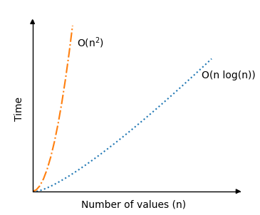
The graph below illustrates how Quicksort significantly reduces time complexity in an average scenario when compared to Bubble, Selection, and Insertion Sort, the preceding sorting algorithms:

Because the array will be split in half fairly evenly each time the Quicksort algorithm calls itself, the recursion portion of the algorithm is actually the reason why the average sorting situation is so quick. Therefore, even if the number of values n doubles, the number of recursive calls does not.
Quicksort Simulation
Use the simulation below to see how the theoretical time complexity O(n2) (red line) compares with the number of operations of actual Quicksort runs.
====EXAMPLE MUKAVU ====
The red line above represents the theoretical upper bound time complexity O(n2) for the worst case scenario, and the green line represents the average case scenario time complexity with random values O(nlog2n).
The average random case situations and the circumstances where the arrays are already sorted differ significantly in terms of Quicksort. You can test it by executing the various simulations mentioned above.
Because of the way it is designed, the already ascending sorted array requires the most element swapping, which accounts for why it requires so many operations. The final element—which is also the largest number—is selected in this instance to serve as the pivot element. In order to place the other values in each sub-array on the left side of the pivot element, where they are previously positioned, they are all switched around.
