Introduction
Runtime
To gain a complete understanding of algorithms, one must be able to assess the runtime, or amount of time an algorithm requires to complete its task.
Investigating an algorithm’s runtime is crucial because utilizing a subpar approach could cause our software to execute slowly or not at all.
Understanding algorithm runtime helps us select the best algorithm for the job, speed up program execution, and manage bigger data sets efficiently.
Actual Runtime
For the following reasons, we will not examine how long an implemented algorithm actually takes to run while evaluating the runtime for various algorithms.
The amount of time an algorithm will really take to execute when it is implemented in a programming language depends on a number of factors:
- The algorithm’s implementation language; the manner in which the programmer prepares the algorithm’s program; the compiler or interpreter used to enable the algorithm’s execution
- the computer’s hardware that the algorithm is operating on
- the computer’s operating system and other processes
- the volume of data that the program is processing
How can we determine one algorithm is faster than another when so many variables affect how long an algorithm takes to execute? A more accurate way to measure runtime must be found.
Time Complexity
It makes more sense to utilize something called temporal complexity to assess and compare various algorithms rather than focusing on an algorithm’s actual runtime.
In contrast to actual runtime, time complexity is more abstract and ignores things like hardware and programming language.
The number of operations required to perform an algorithm on a big volume of data is known as time complexity. Additionally, as the computer requires time for each operation, the number of operations can be thought of as time.
For instance, every value in the array needs to be compared once in the procedure that determines the lowest value in the array. Each of these comparisons can be thought of as an operation, and each operation has a time requirement. Therefore, the amount of values in the array determines how long the process will take in total to discover the lowest value.
As a result, the number of values and the time required to locate the lowest value are linear. There are 100 comparisons for every 100 values, and 5000 comparisons for every 5000 values.
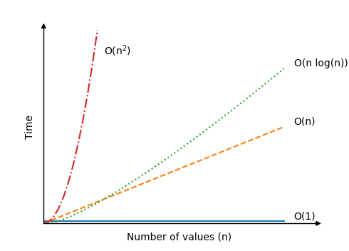
This graph illustrates the linear relationship between time and the number of values in the array:

"One Operation"
When we refer to “operations” in this context, “one operation” could require one or more CPU cycles. In reality, “operation” is merely an abstraction that helps us define time complexity and determine the time complexity of various algorithms.
An algorithm’s “one operation” is any action that we do for every data point or algorithm iteration that requires a fixed amount of time.
For instance, the Bubble Sort algorithm’s comparison of two array elements and subsequent swapping of the larger of the two can be thought of as a single operation. Since Bubble Sort requires a constant amount of time, whether it is seen as one, two, or three processes actually has no bearing on the time complexity.
When an operation takes the same amount of time regardless of the volume of data, we refer to it as “constant time” (n) the algorithm is working through. If an array has 10 or 1000 elements, it takes the same amount of time to compare two specified elements and swap them if one is larger than the other.
Big O Notation
Big O notation is a mathematical notation used to express a function’s upper bound.
Big O notation is primarily used in computer science to determine an algorithm’s worst-case time complexity.
Big O notation uses a capital letter O with parenthesis O(), and inside the parenthesis there is an expression that indicates the algorithm runtime. Runtime is usually expressed using n, which is the number of values in the data set the algorithm is working on.
To help you understand, here are some examples of Big O notation for various algorithms:
| Time Complexity | Algorithm |
|---|---|
Looking up a specific element in an array, like this for example: | |
| Finding the lowest value. The algorithm must do operations in an array with values to find the lowest value, because the algorithm must compare each value one time. | |
Bubble sort, Selection sort and Insertion sort are algorithms with this time complexity. The reason for their time complexities are explained on the pages for these algorithms. Large data sets slows down these algorithms significantly. With just an increase in from 100 to 200 values, the number of operations can increase by as much as 30000! | |
| The Quicksort algorithm is faster on average than the three sorting algorithms mentioned above, with being the average and not the worst case time. Worst case time for Quicksort is also , but it is the average time that makes Quicksort so interesting. We will learn about Quicksort later. |
For various methods, this is how time grows as the number of values n increases:

Best, Average and Worst Case
Big O notation explanations have already discussed “worst case” time complexity, but how can an algorithm have a worst case scenario?
The method that determines which value in an array with n values must noperations to accomplish so, and that is constant. Thus, the best, average, and worst case situations for this algorithm are the same.
However, if we maintain the quantity of values, we shall examine many other strategies.n corrected, the real values may still cause the runtime to vary significantly.
We can appreciate, without getting into the specifics, that a sorting algorithm may have varying runtimes based on the values it is sorting.
Consider the following scenario: you must manually sort 20 numbers from lowest to highest:
8, 16, 19, 15, 2, 17, 4, 11, 6, 1, 7, 13, 5, 3, 9, 12, 14, 20, 18, 10
It will take just a few seconds to complete this.
Consider that you now need to sort 20 data that are nearly sorted:
1, 2, 3, 4, 5, 20, 6, 7, 8, 9, 10, 11, 12, 13, 14, 15, 16, 17, 18, 19
Putting 20 at the end of the list is all it takes to sort the values quickly, isn’t that right?
Algorithms function similarly in that they might be quick or sluggish for the same quantity of data. Thus, in order to evaluate the temporal complexity of various algorithms, we typically use Big O notation to look at the worst-case situation.
Big O Explained Mathematically
This part may be challenging for you to understand, depending on your background in mathematics. Its goal is to give anyone who require a more in-depth explanation of Big O a stronger mathematical foundation.
Do not worry if you do not grasp this right now; you can return at a later time. You may still appreciate the many algorithms in this course, learn how to program them, and comprehend how fast or slow they are, so don’t worry too much if the math is beyond your head.
Big O notation is used in computer science to explain how an algorithm’s runtime grows as the number of data values n rises, and it is used in mathematics to establish an upper bound for a function.
Take into account, for instance, the function:

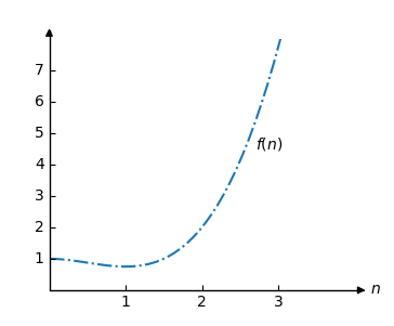
Think of an additional function:
which we can depict as follows:

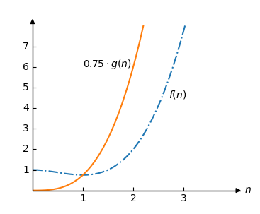
We can choose a constant such that as long as is large enough, thus we can use Big O notation to state that is an upper bound for.
Alright, let’s attempt. We make our decision in such a way.
Let’s now sketch in the same plot:

Since that is the upper bound for any values larger than 1, we clearly observe that.
For the above example to serve as an upper bound, it must be greater than 1. This limit is known as.
Definition
Assume that and have two roles. We state that is the case only in cases when positive constants and other similar
for everybody.
It is acceptable for an algorithm to only be true for a large number of values when evaluating its time complexity because that is when time complexity becomes significant. Stated otherwise, the algorithm’s temporal complexity is not particularly interesting when sorting 10, 20, or 100 items because the machine will sort the values quickly anyhow.
