DSA Bellman-Ford
The Bellman-Ford Algorithm
In a directed network with one or more negative edge weights, the Bellman-Ford algorithm works best for determining the shortest paths between the source vertex and every other vertex.
To achieve this, it iteratively searches every edge in the network for shorter pathways, doing so as many times as there are vertices (minus 1).
==== EXAM MUKAVU ====
Similar to Dijkstra’s method, the Bellman-Ford algorithm can also be applied to graphs with positive edges (both directed and undirected); nevertheless, Dijkstra’s technique is favored in these situations due to its speed.
A graph containing negative cycles will not yield shortest paths when the Bellman-Ford algorithm is applied because a shorter path can always be found by going around in a negative cycle.
We can follow a path in circles called a negative cycle if the total of the edge weights is negative.
Fortunately, negative cycles can be securely detected and reported by using the Bellman-Ford method.
How it works:
1.For the source vertex, put the starting distance to zero; for all other vertices, set the initial distances to infinity.
2.Determine whether a shorter distance can be computed for each edge, then update the distance if it can.
3.Examine every edge (step 2) V−1. periods. This represents the number of times there are vertices (V), less one.
4.Optional: Look for cycles that are negative. Later on, this will be covered in more detail.
The Bellman-Ford algorithm animation above only displays the instances in which verifying an edge results in an updated distance; it does not include the entirety of edge tests that do not.
Manual Run Through
Because the Bellman-Ford algorithm uses the adjacency matrix to check every edge, it is actually very simple to understand. The goal of each check is to determine whether there is a shorter path that can be taken from the vertex on one side of the edge to the vertex on the other side of the edge by walking through the edge.
And all edges have been checked. V−1.periods, with V being the graph’s total vertex count.
The Bellman-Ford algorithm examines each edge in our graph’s adjacency matrix 5-1=4 times in this manner:
==== EXAM MUKAVU ====
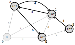
In our graph, the first four edges that are examined are A->C, A->E, B->C, and C->A. The starting vertex of each of these four edges has an infinite distance, so these initial four edge checks do not result in any updates to the shortest distances.
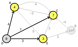
The edges from vertices A, B, and C are examined first, followed by the edges from D. Since vertex D, the starting point, has a distance of 0, the updated distances for vertex D’s edge weights, A, B, and C, are what matter.
The edges that emanate from vertex E should be examined next, as this results in revised distances for vertices B and C.
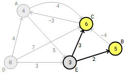
As of right moment, the Bellman-Ford algorithm has examined every edge once. Bellman-Ford checks all edges as many times as there are vertices in the graph, minus one, hence the method will check all edges three more times before it is finished.
The program begins a second round of edge checks, focusing on edges that leave vertex A. A->C and A->E edge checks do not produce updated distances.
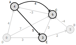
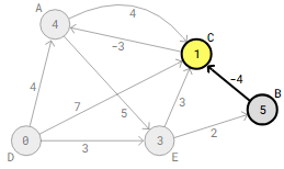
Beyond vertex B, the edge that needs to be examined next is B->C. This results in an updated 5-4=1 distance between vertex D and C.
Vertex A receives an updated distance of 1-3=-2 upon checking the following edge, C->A.
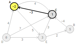
In the second round of the Bellman-Ford method, the edge C->A check is actually the final step that results in an updated distance for this particular graph. The algorithm won’t update any distances and will check every edge twice more.Examining every edge V−1.
The Bellman-Ford algorithm runs a number of times, however this is necessary to ensure that the shortest distances are always obtained.
Implementation of The Bellman-Ford Algorithm
The way we constructed Dijkstra’s algorithm is remarkably similar to how we implemented the Bellman-Ford algorithm.
Using the methods __init__, add_edge, and add_vertex, we first build the Graph class, which will serve as the template for the particular graph on which we will apply the Bellman-Ford algorithm to determine the shortest pathways.
					class Graph:
    def __init__(self, size):
        self.adj_matrix = [[0] * size for _ in range(size)]
        self.size = size
        self.vertex_data = [''] * size

    def add_edge(self, u, v, weight):
        if 0 <= u < self.size and 0 <= v < self.size:
            self.adj_matrix[u][v] = weight
            #self.adj_matrix[v][u] = weight  # For undirected graph

    def add_vertex_data(self, vertex, data):
        if 0 <= vertex < self.size:
            self.vertex_data[vertex] = data
The Graph class also contains the bellman_ford method. This process is used to execute the Bellman-Ford algorithm.
					  def bellman_ford(self, start_vertex_data):
        start_vertex = self.vertex_data.index(start_vertex_data)
        distances = [float('inf')] * self.size
        distances[start_vertex] = 0

        for i in range(self.size - 1):
            for u in range(self.size):
                for v in range(self.size):
                    if self.adj_matrix[u][v] != 0:
                        if distances[u] + self.adj_matrix[u][v] < distances[v]:
                            distances[v] = distances[u] + self.adj_matrix[u][v]
                            print(f"Relaxing edge {self.vertex_data[u]}-{self.vertex_data[v]}, Updated distance to {self.vertex_data[v]}: {distances[v]}")

        return distances
Lines 18–19: Initially, every vertex is assigned an infinitely large distance from the starting vertex, with the exception of the starting vertex, which has a distance of 0.
Line 21: Every edge is examined V−1. periods.
Lines 22–23: The adjacency matrix’s edges are all checked by a double for-loop. Verify the edges that lead to vertices v for each vertex u.
Line 24-26: Update the distance to that vertex v if the edge exists and the computed distance is less than the current distance.
The full code looks like this, which includes the code to perform the Bellman-Ford algorithm and initialize our particular graph:
Example
Python:
					class Graph:
    def __init__(self, size):
        self.adj_matrix = [[0] * size for _ in range(size)]
        self.size = size
        self.vertex_data = [''] * size

    def add_edge(self, u, v, weight):
        if 0 <= u < self.size and 0 <= v < self.size:
            self.adj_matrix[u][v] = weight
            #self.adj_matrix[v][u] = weight  # For undirected graph

    def add_vertex_data(self, vertex, data):
        if 0 <= vertex < self.size:
            self.vertex_data[vertex] = data

    def bellman_ford(self, start_vertex_data):
        start_vertex = self.vertex_data.index(start_vertex_data)
        distances = [float('inf')] * self.size
        distances[start_vertex] = 0

        for i in range(self.size - 1):
            for u in range(self.size):
                for v in range(self.size):
                    if self.adj_matrix[u][v] != 0:
                        if distances[u] + self.adj_matrix[u][v] < distances[v]:
                            distances[v] = distances[u] + self.adj_matrix[u][v]
                            print(f"Relaxing edge {self.vertex_data[u]}-{self.vertex_data[v]}, Updated distance to {self.vertex_data[v]}: {distances[v]}")

        return distances

g = Graph(5)

g.add_vertex_data(0, 'A')
g.add_vertex_data(1, 'B')
g.add_vertex_data(2, 'C')
g.add_vertex_data(3, 'D')
g.add_vertex_data(4, 'E')

g.add_edge(3, 0, 4)  # D -> A, weight 4
g.add_edge(3, 2, 7)  # D -> C, weight 7
g.add_edge(3, 4, 3)  # D -> E, weight 3
g.add_edge(0, 2, 4)  # A -> C, weight 4
g.add_edge(2, 0, -3) # C -> A, weight -3
g.add_edge(0, 4, 5)  # A -> E, weight 5
g.add_edge(4, 2, 3)  # E -> C, weight 3
g.add_edge(1, 2, -4) # B -> C, weight -4
g.add_edge(4, 1, 2)  # E -> B, weight 2

# Running the Bellman-Ford algorithm from D to all vertices
print("\nThe Bellman-Ford Algorithm starting from vertex D:")
distances = g.bellman_ford('D')
for i, d in enumerate(distances):
    print(f"Distance from D to {g.vertex_data[i]}: {d}")
Negative Edges in The Bellman-Ford Algorithm
It defies logic to claim that the Bellman-Ford algorithm discovers the “shortest paths” since negative distances are impossible to depict or imagine. Alternatively, we may state that Bellman-Ford finds the “cheapest paths” in order to simplify the explanation.
In real-world applications, the Bellman-Ford algorithm could assist us in determining delivery routes by providing edge weights that indicate the cost of fuel and other expenses less the profit margin obtained from driving the edge between those two vertices.
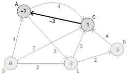
Considering this interpretation, the -3 weight on edge C->A could indicate that we get paid $8 for picking up packages in C and delivering them to A, and that the gasoline cost for the drive from C to A is $5. As a result, we make $3 more than we spend. Consequently, driving the delivery route D->E->B->C->A in our above graph can earn $2 in total.
Negative Cycles in The Bellman-Ford Algorithm
In a graph, we have a negative cycle if we can draw circles and the total of the edges in those circles is negative.
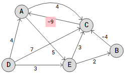
In a graph, we have a negative cycle if we can draw circles and the total of the edges in those circles is negative.
Two negative cycles result from shifting the weight on edge C->A from -3 to -9: A->C->A and A->E->C->A. And the distances we compute and update just get smaller and smaller each time we use the Bellman-Ford technique to verify these edges.
Since we can always travel around again to find a shorter path, the difficulty with negative cycles is that there is never a shortest path.
Implementing the Bellman-Ford algorithm with negative cycle detection is hence beneficial.
Detection of Negative Cycles in the Bellman-Ford Algorithm
Once the Bellman-Ford algorithm has been executed, verify each edge in a graph V by checking 1.The shortest distances are all found at all times.
However, if we examine every edge in one more round and the graph has negative cycles, we should find at least one shorter distance in this final round, right?
Thus, after examining every edge in the Bellman-Ford algorithm, in order to identify negative cycles V−1. All we have to do is examine all the edges one more time, and if this time we discover a smaller gap, we may be certain that there is a negative cycle.
Using the graph above, which has negative cycles because of the C->A edge weight of -9, the bellman_ford method is shown below, along with negative cycle detection:
Example
Python:
					  def bellman_ford(self, start_vertex_data):
        start_vertex = self.vertex_data.index(start_vertex_data)
        distances = [float('inf')] * self.size
        distances[start_vertex] = 0

        for i in range(self.size - 1):
            for u in range(self.size):
                for v in range(self.size):
                    if self.adj_matrix[u][v] != 0:
                        if distances[u] + self.adj_matrix[u][v] < distances[v]:
                            distances[v] = distances[u] + self.adj_matrix[u][v]
                            print(f"Relaxing edge {self.vertex_data[u]}->{self.vertex_data[v]}, Updated distance to {self.vertex_data[v]}: {distances[v]}")

        # Negative cycle detection
        for u in range(self.size):
            for v in range(self.size):
                if self.adj_matrix[u][v] != 0:
                    if distances[u] + self.adj_matrix[u][v] < distances[v]:
                        return (True, None)  # Indicate a negative cycle was found

        return (False, distances)  # Indicate no negative cycle and return distances
Line 30-33: To check for negative cycles, all edges are examined once again.
Line 34: Finding the smallest distances in a graph with negative cycles is illogical (a shorter distance can always be found by examining all edges one more time), hence returning None in place of the shortest distances shows that a negative cycle exists.
Line 36: Returning False indicates that the distances can be returned and that there are no negative cycles.
Returning The Paths from The Bellman-Ford Algorithm
The Bellman-Ford algorithm is being used to determine the overall weight of the shortest paths; for instance, “Distance from D to A: -2” is the outcome.
However, if we keep track of each vertex’s predecessor whenever an edge is relaxed, we can utilize that information later in our code to report the result along with the shortest pathways. This means that in addition to the path weight, we can provide more information in our result: “D->E->B->C->A, Distance: -2”.
The Bellman-Ford algorithm’s whole code is shown in this last code sample, which includes all of the topics we have covered thus far: determining the weights of shortest paths, identifying negative cycles, and determining the shortest paths themselves.
Example
Python:
					class Graph:
    def __init__(self, size):
        self.adj_matrix = [[0] * size for _ in range(size)]
        self.size = size
        self.vertex_data = [''] * size

    def add_edge(self, u, v, weight):
        if 0 <= u < self.size and 0 <= v < self.size:
            self.adj_matrix[u][v] = weight
            #self.adj_matrix[v][u] = weight  # For undirected graph

    def add_vertex_data(self, vertex, data):
        if 0 <= vertex < self.size:
            self.vertex_data[vertex] = data

    def bellman_ford(self, start_vertex_data):
        start_vertex = self.vertex_data.index(start_vertex_data)
        distances = [float('inf')] * self.size
        predecessors = [None] * self.size
        distances[start_vertex] = 0

        for i in range(self.size - 1):
            for u in range(self.size):
                for v in range(self.size):
                    if self.adj_matrix[u][v] != 0:
                        if distances[u] + self.adj_matrix[u][v] < distances[v]:
                            distances[v] = distances[u] + self.adj_matrix[u][v]
                            predecessors[v] = u
                            print(f"Relaxing edge {self.vertex_data[u]}->{self.vertex_data[v]}, Updated distance to {self.vertex_data[v]}: {distances[v]}")

        # Negative cycle detection
        for u in range(self.size):
            for v in range(self.size):
                if self.adj_matrix[u][v] != 0:
                    if distances[u] + self.adj_matrix[u][v] < distances[v]:
                        return (True, None, None)  # Indicate a negative cycle was found

        return (False, distances, predecessors)  # Indicate no negative cycle and return distances

    def get_path(self, predecessors, start_vertex, end_vertex):
        path = []
        current = self.vertex_data.index(end_vertex)
        while current is not None:
            path.insert(0, self.vertex_data[current])
            current = predecessors[current]
            if current == self.vertex_data.index(start_vertex):
                path.insert(0, start_vertex)
                break
        return '->'.join(path)

g = Graph(5)

g.add_vertex_data(0, 'A')
g.add_vertex_data(1, 'B')
g.add_vertex_data(2, 'C')
g.add_vertex_data(3, 'D')
g.add_vertex_data(4, 'E')

g.add_edge(3, 0, 4)  # D -> A, weight 4
g.add_edge(3, 2, 7)  # D -> C, weight 7
g.add_edge(3, 4, 3)  # D -> E, weight 3
g.add_edge(0, 2, 4)  # A -> C, weight 4
g.add_edge(2, 0, -3) # C -> A, weight -3
g.add_edge(0, 4, 5)  # A -> E, weight 5
g.add_edge(4, 2, 3)  # E -> C, weight 3
g.add_edge(1, 2, -4) # B -> C, weight -4
g.add_edge(4, 1, 2)  # E -> B, weight 2

# Running the Bellman-Ford algorithm from D to all vertices
print("\nThe Bellman-Ford Algorithm starting from vertex D:")
negative_cycle, distances, predecessors = g.bellman_ford('D')
if not negative_cycle:
    for i, d in enumerate(distances):
        if d != float('inf'):
            path = g.get_path(predecessors, 'D', g.vertex_data[i])
            print(f"{path}, Distance: {d}")
        else:
            print(f"No path from D to {g.vertex_data[i]}, Distance: Infinity")
else:
    print("Negative weight cycle detected. Cannot compute shortest paths.")
Line 19: The shortest path to each vertex’s predecessor is stored in the predecessors array.
Line 28: Whenever an edge is loosened, the predecessors array is updated with the new predecessor vertex.
Lines 40–49: The shortest path string for each vertex is produced by the get_path method using the predecessors array.
Time Complexity for The Bellman-Ford Algorithm
The Bellman-Ford algorithm’s temporal complexity is mostly determined by its nested loop structure.
The outer for-loop runs V−1 times, V times in case we also have negative cycle detection. For graphs with many vertices, checking all edges one less time than there are vertices makes little difference, so we can say that the outer loop contributes with O(V) to the time complexity.
The two inner for-loops checks all edges in the graph. If we assume a worst case scenario in terms of time complexity, then we have a very dense graph where every vertex has an edge to every other vertex, so for all vertex V the edge to all other vertices V must be checked, which contributes with O(V2) to the time complexity.
Thus, the total time complexity of the Bellman-Ford method is as follows:
O(V3)
However, in practical situations and especially for sparse graphs, meaning each vertex only has edges to a small portion of the other vertices, time complexity of the two inner for-loops checking all edges can be approximated from O(V2) to O(E), and we get the total time complexity for Bellman-Ford
O(V⋅E)
Although the Bellman-Ford approach has a slower temporal complexity than Dijkstra’s algorithm, it is capable of detecting negative cycles and finding the shortest paths in graphs with negative edges, something that Dijkstra’s algorithm is not able to do.
