DSA Graphs
Graphs
A graph is an edge-based and vertice-based non-linear data structure.

In a graph, an edge is used to join two vertices together. A vertex, also known as a node, is a point or an object.
Unlike linear data structures like arrays or linked lists, which only enable us to have one path from one vertex to another, graphs allow us to have multiple paths. This is what makes them non-linear data structures.
When the data consists of items and the interactions between them, graphs are used to represent and solve problems like these:
- Social networks: Friendships and other relationships are the edges, while each individual is a vertex. Potential friends can be suggested via algorithms.
- Maps & Navigation: Roads are kept as edges, and locations, such as towns or bus stations, are saved as vertices. When represented as a graph, algorithms can determine the shortest path between two points.
- The Internet can be visualized as a graph, where hyperlinks are the edges and web pages are the vertices.
- Biology: Neural networks and the spread of diseases are two systems that graphs can simulate.
Graph Properties
To learn about the various Graph features and how they can be combined, watch the animation below.
==== example mukavu ====
An edge-valued graph is known as a weighted graph. An edge’s weight value can be used to represent probability, capacity, duration, or distance.
When every vertex in a graph is connected in some way by edges, the graph is said to be connected. A graph with isolated (disjoint) subgraphs or a single isolated vertex is said to be disconnected.
The edges connecting the pairs of vertices in a directed graph, or digraph, have a direction. An edge’s direction can symbolize concepts like hierarchy or flow.
Whether or not a cyclic graph is directed determines how it is defined:
- A directed cyclic graph is one in which a path that circles the directed edges can be followed. The directed graph in the animation above stops being cyclic when the directed edge from F to G is removed.
- When you can return to the starting vertex without utilizing the same edge more than once, the graph is said to be undirected cyclic. Because we are able to begin and stop in vertebrae C without utilizing the same edge twice, the undirected graph above is cyclic.
An edge that starts and finishes on the same vertex is referred to as a loop, sometimes known as a self-loop. A cycle with just one edge is called a loop. The Graph becomes cyclic when the loop on vertex A in the animation above is added.
Graph Representations
We can learn how a graph is kept in memory by looking at its representation.
Various representations of the graph can:
- occupy more or less room.
- be easier to search or work with more slowly.
- be more appropriate based on the kind of graph we have (weighted, directed, etc.) and the intended use of the graph.
- be simpler to comprehend and use than others.
The various graph representations are briefly introduced below; however, from now on in this tutorial, we will only use the Adjacency Matrix representation for graphs because it is simple to comprehend and use, and it functions in all scenarios that are pertinent to it.
The relationship between neighboring vertices and the direction of the edges connecting them are stored in graph representations. If the edges of a graph are weighted or directed, the graph representations differ slightly.
If there is an edge connecting two vertices, then they are neighboring, or adjacent.
Adjacency Matrix Graph Representation
The graph representation (structure) that we will employ in this tutorial is the adjacency matrix.
The following page illustrates how to put an adjacency matrix into practice.
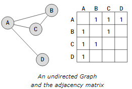
The Adjacency Matrix is a 2D array (matrix) in which the details of the edges connecting vertices i and j are stored in each cell at index (i,j).
The Adjacency Matrix representation is shown next to the graph below.

The numbers in the adjacency matrix above ‘1’ merely indicate the locations of the edges because it depicts an undirected graph. Because the edges in the adjacency matrix are bidirectional (an undirected graph), the values within it are symmetrical as well.
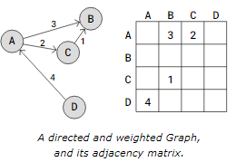
We must choose which vertices the edges go from and to by putting the value at the appropriate indexes (i,j) in order to form a directed graph with an adjacency matrix. In the adjacency matrix, we can enter values other than ‘1’ to represent a weighted graph.
A directed and weighted graph is shown here, along with the Adjacency Matrix representation.

The value 3 on index (0,1) in the adjacency matrix above indicates that there is an edge from vertex A to vertex B, and that edge has weight 3.
As you can see, the adjacency matrix for a directed graph does not need to be symmetric; the weights are simply inserted into it for the appropriate edge.
Adjacency List Graph Representation
When dealing with a “sparse” graph that has a number of vertices, employing an adjacency list instead of an adjacency matrix can save space because the latter would allocate a lot of memory on empty array members for nonexistent edges.
A “sparse” graph is one in which the edges connecting each vertex to the other vertices in the graph are limited to a small percentage.
Every vertex in a graph has a Linked List (or Array) with its edges, and an Adjacency List has an array with all of the vertices in the graph.

The vertices A through D are arranged in an array in the adjacency list above, and each vertex in the array has its index written immediately next to it.
A pointer to a linked list that represents each vertex’s edges is present in every vertex of the array. To be more precise, the neighboring vertices’ indexes are contained in the Linked List.
For instance, a link to a Linked List with the values 3, 1, and 2 is present at vertex A. These numbers represent the indexes to vertices D, B, and C that are close to A.
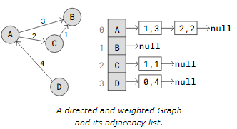
A directed and weighted graph can alternatively be represented by an adjacency list, as in this example:

Vertices in the aforementioned Adjacency List are kept in an Array. A pointer to a linked list with edges encoded as i,w, where w is the weight of the edge and i is the index of the vertex it goes to, is present in each vertex.
An example of a linked list with an edge to vertex A is found at node D. The numbers 0,4 indicate that vertex D and vertex on index 0 (vertex A) have an edge with a weight of 4.
